Core Tutorials

1. Basics
2. Equations
3. Loops and Modules
4. Graphics
5. Working with Data

Examples

• Coupled Oscillators
• Conformal Mapping Transformation
• Finite Quantum Well

Advanced

• Creating a Publishable Figure
• Advanced Drawing Options

Coupled Oscillators

Simple Case in 1 dimension

First lets solve the simple harmonic motion problem. $\frac{d^2 x(t)}{dt^2}=-x(t)$ This yields the cosine and sine terms that are soo familiar.

DSolve[ x''[t] == -  x[t], x[t], t]

Note the integration constants are output in Mathematica as C[1] and C[2].

2 dimensional coupled oscillation

Now lets do something a bit more interesting! How about a two dimensional coupled oscillator?

$\frac{d^2 x(t)}{dt^2}= -a_1 x(t)+a_3 y(t)$ $\frac{d^2 x(t)}{dt^2}= -a_3 y(t)+a_2 x(t)$

This system has real solutions when Det[{{a1,a3},{a3,a2}}]>=0 Lets just pick some semi-random coefficients and let DSolve do the hard work for us

eq1 = x''[t] == -8. x[t] + 2 y[t]
eq2 = y''[t] == -  1. y[t] + 2 x[t]
DSolve[ {eq1, eq2}, { x[t], y[t]} , t] // Chop // Flatten

We can diagonalize the matrix equation using Eigensystem. The first list in Eigensystem is the eigenvalues and the second is the eigenvectors. Taking the square root of the eigenvalues will give the frequencies of oscillation.

Eigensystem[{{ 8., 2}, { 2, 1}}]
Sqrt[First[Eigensystem[{{ 8., 2}, { 2, 1}}]]]

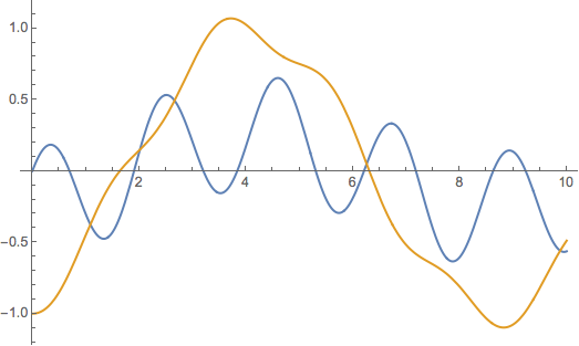
Now lets add initial conditions to the system and plot the resulting motion.

sol = Simplify[Chop[
  DSolve[ {eq1, eq2, x[0] == 0, x'[0] == 1, y[0] == -1, 
    y'[0] == 0  }, { x[t], y[t]} , t]]]
Plot[ Evaluate[{ x[t], y[t]} /. sol], {t, 0, 10}]

Solving a nonlinear system

This was a nice problem to show how quickly a mildly complex physics problem can be solved quickly using Mathematica. This is great, but computers can do much more than humans can when it comes to numerical calculation. Lets now try to solve a much more complex set of nonlinear coupled equations

$\frac{d^2 x(t)}{dt^2}= -a_1 x(t)+a_3 y(t)^2$ $\frac{d^2 x(t)}{dt^2}= -a_3 y(t)^2 + a_2 x(t)^2$

eq1 = x''[t] == -8. x[t] + 2 y[t]^2
eq2 = y''[t] == -  y[t]^3 + 2 x[t]^2
DSolve[ {eq1, eq2}, { x[t], y[t]} , t] // Chop // Flatten

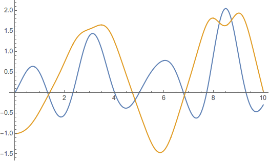
Note that this much more complicated non - linear oscillation is not solved by DSolve, it is simply returned in the output. This means that Mathematica cannot find a closed form solution to the differential equations. This should not worry you too much, as we can use the numerical version of DSolve to find the resulting motion.

sol = NDSolve[ {eq1, eq2, x[0] == 0, x'[0] == 1, y[0] == -1, 
      y'[0] == 0  }, { x[t], y[t]} , {t, 0, 10}] // Chop // Flatten;
Plot[ Evaluate[{ x[t], y[t]} /. sol], {t, 0, 10}]

Further Reading

• Mathematica Documentation
• Computable Document Player