Core Tutorials
Examples
Advanced
Creating a figure for publication
There are a number of options that you should set when you are making a figure using Mathematica. While the default plot options make very nice looking plots when viewed on a computer monitor, the labels and lines are not easily read when printed on paper. This can be fixed by setting plot options
rand:=RandomReal[NormalDistribution[0,0.05]];
testFunc:=Exp[-(x-m)^2/2s^2]/.{m->0,s->1};
sampleData=Table[{x,rand+testFunc},{x,-3,3,0.001}];

plt1=ListPlot[sampleData,
PlotStyle->RGBColor[235/256,174/256,27/256],
PlotRange->{{-3,3},{0,1.2}},
Frame->True,
Axes->False,
FrameStyle->Directive[Thickness[0.003],Black,16],
FrameTicksStyle->Directive[Thickness[0.004]],PlotLabel->Style["Plot Title \[Alpha]",24,Black,FontFamily->"Arial"],
FrameLabel->{
{Style["y axis \[Gamma]",16,FontFamily->"Arial"],
None},
{Style["x axis \[Beta]",16,FontFamily->"Arial"],
None}},
AspectRatio->.7,
ImageSize->600];

plt2=Plot[testFunc,{x,-3,3},
PlotStyle->{Blue,Thickness[0.005]}
];

text1=Graphics[Text[Style["param 1 = 0.5\[Mu]m\nparam 2 = 5.2 s",16],{-2,1}]];

Show[plt1,plt2,text1]
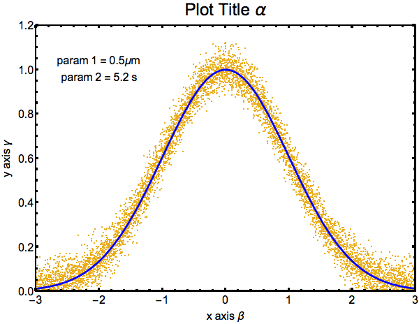
Now you should be able to see all of the lines and ticks clearly!
Saving the graphic
tldr: save as PDF!
After you have made a well labeled and easily read figure you will need to save it. This can be handled in two ways:
- Right click on the figure and select “Save Graphic As…”
- Use the
Exportfunction to save the plot to file.
When saving you should make sure you are saving the figure in a vectorized image format (EPS or PDF). Many journals only accept figures in a vectorized format and you cannot create a vector image from a JPEG, so be sure to do this! Many find saving figures in PDF format to be easier than EPS, as they have a PDF viewing program installed on their computer anyways (which you should).