Advanced Graphics Tutorial

## Visualizing a Probability Distribution Function Building off of the lectures Patrick gave on graphics, let’s illustrate the concepts using some examples which came up in research. Let’s say that you want to model some histogram by a Johnson SU PDF. Don’t know what that is? Google it!

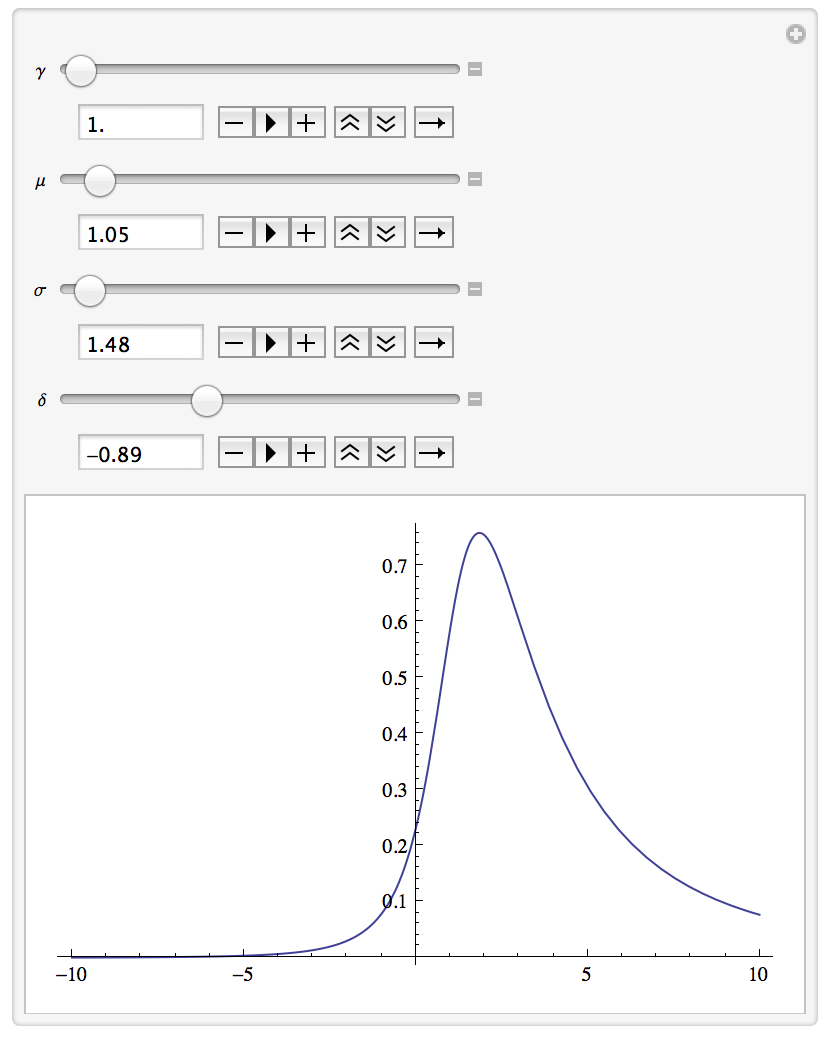
Now we want to know what the parameters of the Johnson function do to its shape. How can we do that in real time? Let’s use Manipulate.

Manipulate[
 Plot[E^(-(1/
    2) (\[Gamma] + \[Delta] ArcSinh[(x - \[Mu])/\[Sigma]])^2)/Sqrt[
  1 + (x - \[Mu])^2/\[Sigma]^2], {x, -10, 10}], {\[Gamma], 1, 
  10}, {\[Mu], 0, 20}, {\[Sigma], 1, 20}, {\[Delta], -3, 3}]

Manipulate of Johnson

Note, I’ve not included the normalization here, but you can certainly add it in. What’s the difference between an SU and SB Johnson?

Mock Up of Silicon Strip Detector

Let’s use Mathematica to make a mock up of one of the Upgrade Tracker planes for the LHCb detector. This would be useful for visualizing locations of hits in the detector itself.

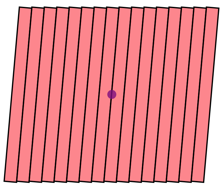
Let us model one plane as a collection of staves, which each stave being modeled as a rectangle. This rectangle should have length 1336 mm. The total width of the plane is 1528 mm, and is composed of 16 staves. To complicate things, the u and v planes have each of these staves rotated at 5 degrees from the vertical. Let’s draw this.

\[Theta] = -5 \[Pi]/180;(*convert to radians*)
utstartx = 1526/2.;
utstarty = 1336/2.;

We’ll use the utstartx and ut start y at these locations to make sure the detector is centered around zero.

Now, we can make a table of one stave at different positions, and rotate that graphic.

utUplane = Graphics[Table[{EdgeForm[Thick], Red, Opacity[0.5], 
   GeometricTransformation[
    Rectangle[{-utstartx + 
       t*(utstartx/8), -utstarty}, {-utstartx + (t + 1) (utstartx/8), utstarty}], 
    RotationTransform[\[Theta], {1/16 (-15 + 2 t) utstartx, 0}]]}, 
    {t,0, 15}]]

Here, we have one rectangle, with a starting x which is indexed by the parameter t. We make a table of these, then rotate each one using RotationTransform by our angle theta around the center of the stave itself.

Now to make the whole thing a bit more realistic, let’s add the beampipe in the picture, which has diameter 68.8 mm.

beampipe = Graphics[{Purple, Opacity[0.8], Disk[{0, 0}, 68.8/2]}];

Show[{utUplane,beampipe}]

UT u plane

Core Tutorials

Examples

Advanced

Advanced Graphics Tutorial

Mock Up of Silicon Strip Detector

Further Reading